Chapter 6. Analysis of data and curves
Fast Fourier Transform
This function can be accessed by the command FFT.... It can be found in the Analysis Menu when a table or a plot is selected. The Fourier transform decomposes a signal in its elementary components by assuming that the signal x(t) can be describe as a sum:

in which  are the frequencies, an are the amplitudes of each frequency and
  are the phase corresponding frequency. SciDAVis will compute these parameters and build a new plot of the amplitude as a function of the frequency.
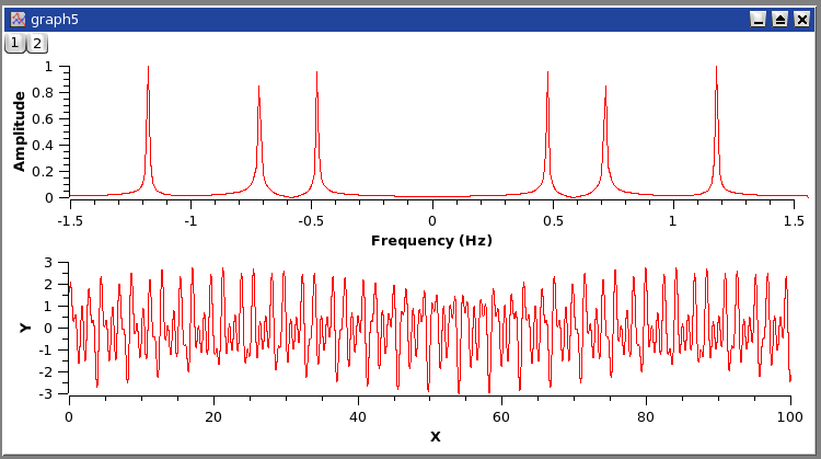
Figure 6-1. An example of a inverse FFT.
FFT performed on a curve to extract the characteristic frequencies. The signal is on the bottom plot, while the amplitude-frequency plot is on the top layer. In this example, the amplitude curve has been normalized, and the frequencies have been shifted to obtain a centered x-scale.
Some parameters of the FFT can be modified in the FFT dialog.