The SciDAVis Handbook
Prev	Chapter 3. Command Reference	Next

The Analysis Menu

The commands which are available in this menu are not the same if a table or a plot is selected.

Commands for the analysis of data in tables

Statistics on Columns

Creates a new table providing basic statistical information about the selected columns in the active table: average, variance, standard deviation, max value, etc...

You can select several columns in one table, one line will be created for each column. You can't select columns in different tables to obtain one single table of statistics.

Statistics on Rows

Creates a new table providing basic statistical information about the selected rows in the active table: average, variance, standard deviation, max value, etc...

See the Statistics on Columns command command for more details.

Sort Column

Sorts the columns selected. If more than one column is selected, you can sort them:

separately: each column will be sorted in ascending or descending order
together: the column selected as leading column will be sorted in ascending or descending order, and the others column selected will be sorted in order to keep the rows unchanged.

Sort Table

This is the same command as Sort Column but it operate on all columns of the active table.

Normalize

Normalizes the columns selected, that is modify the data in order to obtain a range of 0 to 1. All columns selected are normalized separately. This command doesn't create new normalized columns but replace the values of the selected columns.

Normalize -> Columns: Normalizes the selected column.
Normalize -> Table: Normalizes all the columns of the table, it is not a global normalization of all values of the table: each column is normalized separately.

FFT...

Computes a direct or inverse Fast Fourier Transform. The parameters used can be set with the FFT dialog. See the fft section of the Analysis chapter for more details.

Correlate

Does a cross-correlation of the two columns which are selected. See the correlate section of the Analysis chapter for more details.

Convolute

Does a convolution of the two columns which are selected. The first one being the response and the second the signal. See the convolution section of the Analysis chapter for more details.

Deconvolute

Does a deconvolution of the two columns which are selected. The first one being the response and the second the signal. See the deconvolution section of the Analysis chapter for more details.

Non Linear Curve Fit... (Ctrl-Y)

Opens the Non-linear Fit dialog, allowing you to choose the curve to fit, the algorithm and the tolerance, the number of iterations to be performed, and to type the analytical function to use, the names of the fitting parameters and their initial guessed values. See the Non Linear Curve Fit section of the Analysis chapter for more details.

Commands for the analysis of curves in plots

The following items are enabled only if the active window is a 2D Multilayer Plot Window. If the active plot layer contains more than one curve, and the Data Range Selectors are not enabled, a dialog window will pop-out allowing you to select the curve you want to analyse.

In most of the cases (except for integration), a new red curve is added to the active plot layer and a a new table containing the data used to plot this curve is added to the workspace. Useful information about the operation performed will be showed in the Results Log display.

The commands FFT... and Non Linear Curve Fit... are presented in the Table Analysis Menu.

Analysis -> Differentiate

Creates a new plot displaying the resulting curve of the numerical differentiation. The computation of the derivative is done by centered finite diferences.

This command creates a new table which contains one column for X-values and one column for derivatives of Y-values. It also creates a new plot of the derivative.

Analysis -> Integrate...

Opens the Integration dialog, allowing to choose the curve to integrate and the integration method.

This command can't be used to obtain a cumulative curve from a selected curve, it can only compute the integral of the data between two limits. The result is given in the Log Panel.

Analysis -> Smooth

Savitski-Golay

This command performs a smoothing of the selected curve with the Savitzky-Golay method. The formula used to smooth the curve defined by the points y_i=f(x_i) is:

The f_i values are computed by fitting the data points to a polynome, they depend on the number of points used for the smoothing of the curve and the order of the polynome. Compared to the moving window average method, the advantage of this smoothing method is that the values of extrema are not truncated. The dialog allows to specify the curve which will be smoothed, the value of the order of the polynome, the number of data points used for the polynomial fit before and after each point and the color used to draw the smoothed curved. A new table will be created to store the data points x_i, z_i.

Figure 3-1. The Smooth -> Moving Window Average... dialog.

Moving Window Average...

This command performs a smoothing of the selected curve with the moving window average method. The formula used to smooth the curve defined by the points y_i=f(x_i) is:

The greater the number of points n, the smoother the resulting curve z_i=f(x_i) is. The dialog allows to specify the curve which will be smoothed, the value of n and the color used to draw the smoothed curve. A new table will be created to store the data points x_i, z_i.

Figure 3-2. The Smooth -> Moving Window Average... dialog.

Analysis -> FFT Filter

Low Pass...

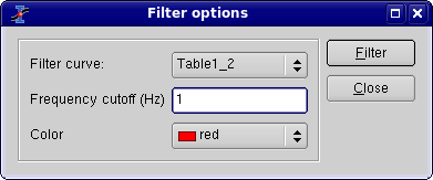
This command allows to filter the high frequencies of a signal. See the filtering section for more details. A dialog box will be opened in which you can select the curve to filter and the cut-off frequency of the filter.

Figure 3-3. The FFT Filter -> Low Pass... dialog.

This command creates a new table with the filtered data, and a new curve will be added on the current plot.

High Pass...

This command allows to filter the low frequencies of a signal. See the filtering section for more details. A dialog box will be opened in which you can select the curve to filter and the cut-off frequency of the filter.

Figure 3-4. The FFT Filter -> High Pass... dialog.

This command creates a new table with the filtered data, and a new curve will be added on the current plot.

Band Pass...

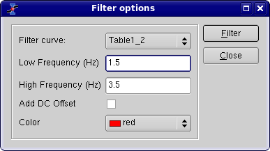
This command allows to filter the low and high frequencies of a signal. See the filtering section for more details. A dialog box will be opened in which you can select the curve to filter and the cut-off frequency of the filter.

Figure 3-5. The FFT Filter -> Band Pass... dialog.

This command creates a new table with the filtered data, and a new curve will be added on the current plot.

Band Block...

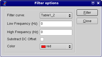
This command allows to keep the low and high frequencies of a signal. See the filtering section for more details. A dialog box will be opened in which you can select the curve to filter and the cut-off frequency of the filter.

Figure 3-6. The FFT Filter -> Band Block... dialog.

This command creates a new table with the filtered data, and a new curve will be added on the current plot.

Analysis -> Interpolate...

Performs an interpolation. The curve must have enough data points to compute the interpolated points, if not a warning message will be prompted out.

The methods available to perform the interpolation are Linear (the curve must contain at least 3 points), Cubic Spline (the curve you analyse must contain at least 4 points, if not a warning message will be prompted out, Non-rounded Akime spline (the curve you analyse must contain at least 5 points). See the Analysis chapter for a comparison of the differents methods.

Figure 3-7. The Interpolate... dialog.

This command creates a new curve on the current plot, and a new table.

Analysis -> FFT...

Performs a forward or inverse FFT transform of the selected curve. The parameters used can be set with the FFT dialog.

The inverse FFT transform of a forward transform will result in a data set identical to that used for the forward transform.

Analysis -> Fit Linear

Performs a linear fit of the selected curve. The results will be given in the Log panel

Analysis -> Fit Polynomial...

Opens the Polynomial Fit dialog, allowing you to choose the curve to fit, the order of the polynomial function to use, the number of points of the resulting curve and the abscissae limits for the fit.

Analysis -> Fit Exponential Decay

First Order...: Opens the Exponential Fit dialog, allowing you to choose the curve to fit and the initial guesses for the fit parameters.
Second Order...: Opens a dialog, allowing you to choose the curve to fit and the initial guesses for the fit parameters.
Third Order...: Opens a dialog, allowing you to choose the curve to fit and the initial guesses for the fit parameters.

Analysis -> Fit Exponential Growth...

Performs an exponential growth fit of the selected curve.

Analysis -> Fit Lorentzian

Performs a lorentzian fit of the selected curve. It can be used to obtain a correlation equation of a bell shaped data set.

Analysis -> Fit Gaussian

Performs a gaussian fit of the selected curve.It can be used to obtain a correlation equation of a bell shaped data set.

Analysis -> Fit Bolzmann (sigmoidal)

Performs a fit to a bolzmann function of the selected curve. It can be used to obtain a correlation equation of a S shaped data set.

Analysis -> Fit Multi-peak ->Gaussian...

Performs a fit to a sum of N gaussian functions of the selected curve.

Analysis -> Fit Multi-peak -> Lorentzian...

Performs a fit to a sum of N lorentz functions of the selected curve.

Prev	Home	Next
The Data Menu	Up	The Table Menu